


There are several risk assessment method kinds (ISO 14121-2 points 4 of them) and multitude of actual methods — is there any reason to thing about another one?
Machinery risk assessment is (usually) related to control system performance levels (PL), as defined in ISO 13849-1. The standard presents a simple graph (“the graph”), used to determine required PL, starting from potential severity of injury (S), exposure frequency or time (F) and possibility of avoiding the hazard (P). While the graph is pretty simple, any risk assessment concerning safety functions and PL-s should stick somehow to these estimations. In particular, having a system evaluating to “PL e” and safeguarding compliant to PL e, the overall risk assessment should result in “safe”.
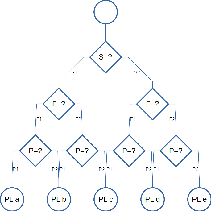
1 and 2 represent low/high (whatever it means) values respectively.
Extending the graph to include expected safeguarding, would lead nowhere (i.e. to a huge, tangled and error prone result). As an alternative, the graph can be transformed to equivalent numerical variables S, F and P. Then, the raw risk[1]risk of hypothetical machinery with no safety means, a.k.a. “primary” will be:
Rr = S × F × P.
The raw risk is a base to choose the required performance level (PLr) of the safety related control system. To get the actual risk (Ra), Rr will be multiplied by other factors, e.g. control system performance (C), depending on the actual PL:
Ra = Rr × C.
The Ra evaluation (acceptable or not) and assigning Rr to PL should be coherent. Risk that is equivalent to PL a can be considered acceptable,[2]this is a kind of contradiction, as requiring PL a is requiring risk reduction; but otherwise, we would have to introduce more states, i.e. a risk lower than (S1,F1,P1) combination as in the table below:
| PL | risk evaluation |
| a | acceptable |
| b | conditionally acceptable[3]the goal of risk evaluation is a binary decision: yes/no, further risk reduction is necessary or not; therefore, “conditionally acceptable” means “not acceptable, yet we just need/can add … Continue reading |
| c | conditionally acceptable |
| d | not acceptable |
| e | not acceptable |
PFHd
According to ISO 13849-1, performance level is (together with some other measures) average probability of dangerous failure per hour, PFHd.
| PL | PFHd less than | PFHd more or equal to |
| a | 1E-4 | 1E-5 |
| b | 1E-5 | 3E-6 |
| c | 3E-6 | 1E-6 |
| d | 1E-6 | 1E-7 |
| e | 1E-7 | 1E-8 |
Relation between PFHd and PL.
Factors’ values
We assume:
S1 = 1,
F2 = 1,
P2 = 1.
S is the only variable, that can be above 1. All the others will scale the risk down, i.e. their values are between 0 (exclusive) and 1 (inclusive).
The other sides we name:
s := S2,
f := F1,
p := P1.
Thus, the range of R is from f×p (S1×F1×P1) to s (S2×F2×P2).
Considering the PFHd values corresponding to PL a and PL e, the proportion f×p:s is between 10⁻⁷:10⁻⁵ and 10⁻⁸:10⁻⁴, i.e. 1:100 to 1:10,000, average 1:1000[4]the scale is logarithmic, so “average(a,b)” means √(a×b) :
s / f × p ≈ 1000.
The two paths: (S1, F2, P2) and (S2, F1, P1) result in PL c. Therefore, the two products should be close: s×f×p and 1×1×1, i.e.:
s × f × p ≈ 1.
Considering PL b or PL d, the sub-paths (F1, P2) and (F2, P1) lead to same PL:
f ≈ p.
If “≈” were “=”, the above equations would result in: s = 10√10 ≈ 31.6, f = p = 1/√s ≈0.18. Fortunately, it is not; so we can look for some other values, close but nicer (easy to remember).
40 : 0.2 : 0.2
Looks good! The threshold values (maximum R belonging to a given PL) could be: 0.08, 0.4, 2, 10.
Disadvantage: frequency 0.2 events per hour is about 2/shift; we would like the f to be lower, as the frequency is a factor to vary.
20: 0.1 : 0.2
We find the set s = 20, f = 0.1, p = 0.2 as optimum. Minimum frequency 0.1 event per hour is ca. once a day (or once a shift).
The corresponding threshold values could be: 0.03, 0.3, 1.5, 10, i.e.:
| PL | R more than | R less or equal to |
| a | – | 0.03 |
| b | 0.03 | 0.3 |
| c | 0.3 | 1.5 |
| d | 1.5 | 10 |
| e | 10 | – |
The following table is equivalent to the graph.
| S | F | P | Rr | PLr |
| 1 | 0.1 | 0.2 | 0.02 | a |
| 1 | 0.1 | 1 | 0.1 | b |
| 1 | 1 | 0.2 | 0.2 | b |
| 1 | 1 | 1 | 1 | c |
| 20 | 0.1 | 0.2 | 0.4 | c |
| 20 | 0.1 | 1 | 2 | d |
| 20 | 1 | 0.2 | 4 | d |
| 20 | 1 | 1 | 20 | e |
Control system performance factor C
Having a safety function (e.g. an interlocking guard stopping the hazard movement), the risk will be scaled down — according to the function performance level. The straightforward approach is to keep the proportion between the PL’s PFHd, i.e. PL e should diminish the risk 10 times more than PL d. Moreover, the lowest PFHd (1E-4) can be considered as changing nothing: C(PL a) = 1. We assume:
C = PFHd × 10000,
or — if PFHd is not known — the following (PL’s upper range times 10000):
| PL | C |
| a | 1 |
| b | 0,1 |
| c | 0,03 |
| d | 0,01 |
| e | 0,001 |
Copyright
The presented method is free, the only obligation is to keep the name “iterum” and the source “ocena-ryzyka.pl”.